doc22940 · May 10, 2020 22:24 · Nov 25, 2019 · Nov 25, 2019 · Nov 25, 2019 · Nov 25, 2019
diff --git a/README.md b/README.md
@@ -82,6 +82,7 @@ Finally, we can use [ndjson-cli](https://github.com/mbostock/ndjson-cli), [geopr
 npm install -g ndjson-cli d3-geo-projection
 
 # Scale the coordinates to fit in a 1000x600 box
+# reflectY(true) because SVGs count from top to bottom
 geoproject 'd3.geoIdentity().reflectY(true).fitSize([1000, 600], d)' < thomas.geojson > rescaled.geojson
 
 # Convert GeoJSON to newline-delimited JSON
@@ -93,7 +94,7 @@ ndjson-cat rescaled.geojson | ndjson-split 'd.features' > rescaled.ndjson
 geo2svg -n -w 1000 -h 600 -p 3 rescaled.ndjson > thomas.svg
 ```
 
-`thomas.svg` will have 43 paths, each representing a perimeter of the Thomas fire! Here's what it looks like in Illustrator:
+Because we converted the file to newline-delimited JSON before feeding it to `geo2svg`, the resulting `thomas.svg` will have 43 paths instead of combining all features into one path, and each one will have the timestamp `id` attribute, which makes it visible in places like Illustrator:
 
 ![Illustrator screenshot](https://user-images.githubusercontent.com/2120446/69543285-2855cc80-0f85-11ea-9011-a2cdba164359.png)
 

diff --git a/README.md b/README.md
@@ -46,13 +46,23 @@ We can do pretty much everything using a few commands if we first install [Node.
 
 First, we'll combine our long list of downloaded shapefiles into one file with GDAL.
 
+GDAL lets you combine multiple layers together like so:
+
+```sh
+# Start with first layer
+ogr2ogr combined.shp input.shp
+
+# Add additional layer
+ogr2ogr -update -append combined.shp input2.shp -nln combined
+```
+
+We can generalize this in a loop, where we create `combined.shp` with the first file in our list, and append the rest:
+
 ```sh
 # Loop through the files and add them to combined.shp
 for f in *.shp; do if [ -f combined.shp ]; then ogr2ogr -update -append combined.shp $f -nln combined; else ogr2ogr combined.shp $f; fi; done
 ```
 
-Note: the tortured if/else syntax is only because we need to create a file with the first layer and then merge the remaining ones in.
-
 Next, we'll convert the combined shapefile into a GeoJSON file. We'll also reproject the file to California State Plane Zone 5, which seems like a good option for display given the location of the fire in Southern California.
 
 ```sh

diff --git a/README.md b/README.md
@@ -198,3 +198,8 @@ We could also modify this script to generate multiple SVGs instead of one, or ge
 ## Option 3: Use QGIS
 
 You can also use [QGIS](https://www.qgis.org/en/site/) for some or all of these steps. You can reproject your coordinates, combine the shapefiles into one file, or convert it GeoJSON. You can also use the Print Composer to export an SVG without ever leaving QGIS, but it can be a bit tricky to get exactly what you want.
+
+## Useful links
+
+- [GDAL cheatsheet](https://github.com/dwtkns/gdal-cheat-sheet) by Derek Watkins
+- [Command-Line Cartography](https://medium.com/@mbostock/command-line-cartography-part-1-897aa8f8ca2c) by Mike Bostock
diff --git a/README.md b/README.md
@@ -65,14 +65,14 @@ ogr2ogr thomas.geojson -f "GeoJSON" -lco id_field=perDatTime -t_srs "EPSG:2229"
 
 Note: with enough layers, the resulting GeoJSON file could be gigantic - if needed you can reduce the output file size by adding `-lco coordinate_precision=[number of digits]`.
 
-Finally, we can use [ndjson-cli](https://github.com/mbostock/ndjson-cli), [geoproject](https://github.com/d3/d3-geo-projection#geoproject), and [geo2svg](https://github.com/d3/d3-geo-projection#geo2svg) to turn this GeoJSON file into a 1000x1000 SVG with a path element for each timestamped perimeter.
+Finally, we can use [ndjson-cli](https://github.com/mbostock/ndjson-cli), [geoproject](https://github.com/d3/d3-geo-projection#geoproject), and [geo2svg](https://github.com/d3/d3-geo-projection#geo2svg) to turn this GeoJSON file into a 1000x600 SVG with a path element for each timestamped perimeter.
 
 ```sh
 # Install dependencies
 npm install -g ndjson-cli d3-geo-projection
 
-# Scale the coordinates to fit in a 1000x1000 box
-geoproject 'd3.geoIdentity().reflectY(true).fitSize([1000, 1000], d)' < thomas.geojson > rescaled.geojson
+# Scale the coordinates to fit in a 1000x600 box
+geoproject 'd3.geoIdentity().reflectY(true).fitSize([1000, 600], d)' < thomas.geojson > rescaled.geojson
 
 # Convert GeoJSON to newline-delimited JSON
 # We have to do this to get one path per feature in our resulting SVG

diff --git a/README.md b/README.md
@@ -31,7 +31,8 @@ Once we have the files, we need to do a few things:
 
 1. Consolidate all the individual shapefiles into a single file with one layer for each timestamp
 2. Reproject the file to the desired coordinate system for display (optional)
-3. Convert the file from a shapefile or GeoJSON file into an SVG
+3. Scale the coordinates down to our desired output size
+4. Convert the coordinate data into an SVG
 
 We'll briefly cover three different methods for this:
 

diff --git a/README.md b/README.md
@@ -8,7 +8,7 @@ This index page contains links to a series of shapefiles of the fire boundary, e
 
 https://rmgsc.cr.usgs.gov/outgoing/GeoMAC/2017_fire_data/California/Thomas/
 
-There are a total of 387 files representing 43 timestamps, because each individual timestamp has a shapefile that consists of 8 files with different extensions, plus an additional .zip file version of those files.
+There are a total of 387 files representing 43 timestamps, because each individual timestamp has a shapefile that consists of 8 files with different extensions, plus an additional .zip file version of those files. (There's also a bit of data for January 2018, but we'll just use the 2017 files)
 
 ## Download all the files
 

diff --git a/README.md b/README.md
@@ -84,7 +84,7 @@ geo2svg -n -w 1000 -h 600 -p 3 rescaled.ndjson > thomas.svg
 
 `thomas.svg` will have 43 paths, each representing a perimeter of the Thomas fire! Here's what it looks like in Illustrator:
 
-![Illustrator screenshot](./illustrator.png)
+![Illustrator screenshot](https://user-images.githubusercontent.com/2120446/69543285-2855cc80-0f85-11ea-9011-a2cdba164359.png)
 
 Putting all of the steps together in one script, we end up with:
 
@@ -190,7 +190,7 @@ node generate-svg.js
 
 It will produce a `thomas.svg` file with one path for each fire perimeter, and an ascending color scale that makes it a little easier to see the progression when opened in Illustrator: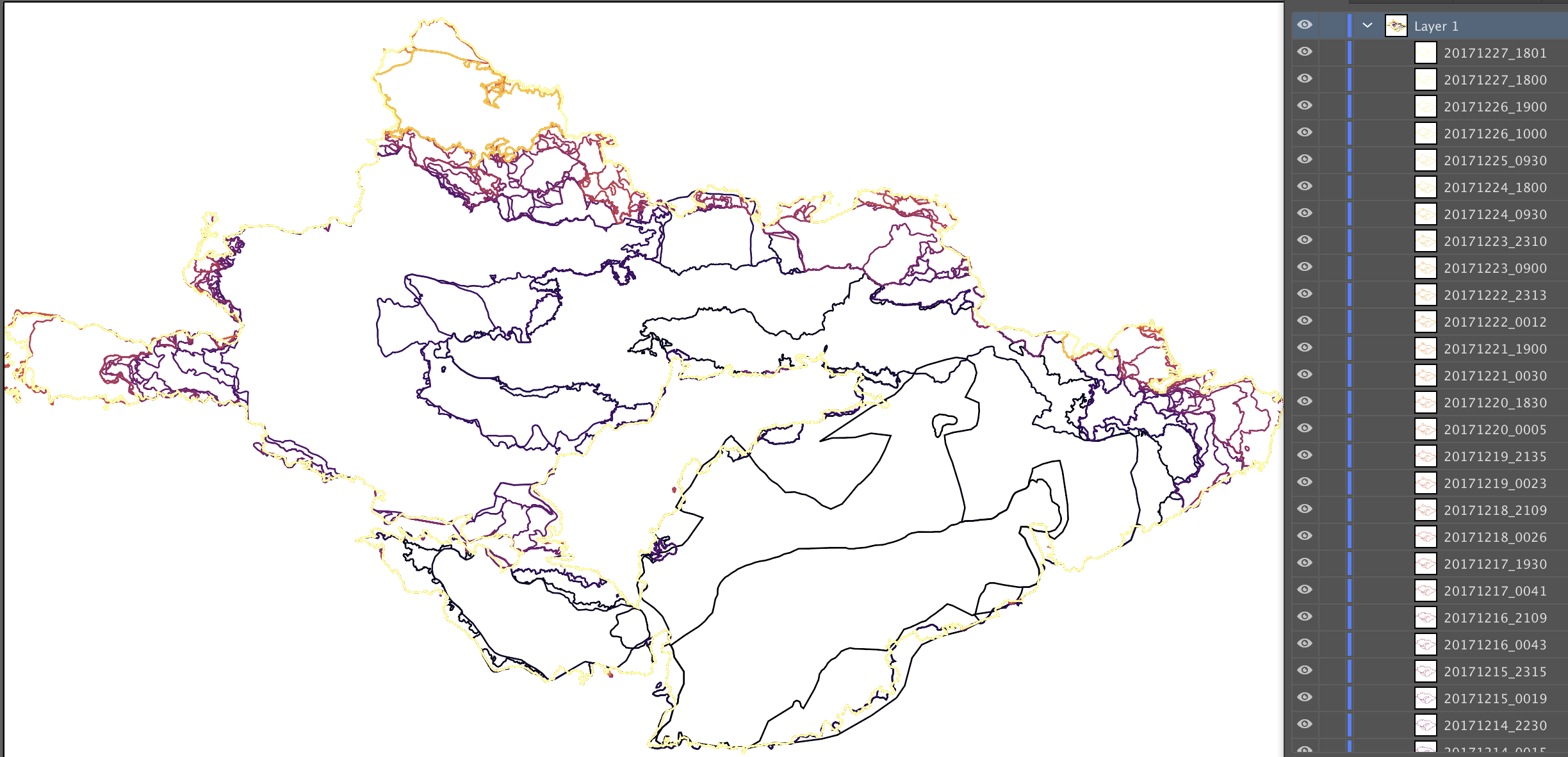
 
-![Illustrator screenshot 2](./illustrator-2.png)
+![Illustrator screenshot 2](https://user-images.githubusercontent.com/2120446/69543284-2855cc80-0f85-11ea-9bcd-bc2d2ce1cc31.png)
 
 We could also modify this script to generate multiple SVGs instead of one, or generate raster images at various sizes, or other fun things.
 

diff --git a/illustrator-2.png b/illustrator-2.png
diff --git a/illustrator.png b/illustrator.png
diff --git a/README.md b/README.md
@@ -8,7 +8,7 @@ This index page contains links to a series of shapefiles of the fire boundary, e
 
 https://rmgsc.cr.usgs.gov/outgoing/GeoMAC/2017_fire_data/California/Thomas/
 
-There are a total of 387 files representing 43 timestamps, because each individual timestamp has a shapefile that consist of 8 files with different extensions, plus an additional .zip file version of those files.
+There are a total of 387 files representing 43 timestamps, because each individual timestamp has a shapefile that consists of 8 files with different extensions, plus an additional .zip file version of those files.
 
 ## Download all the files
 
@@ -46,25 +46,28 @@ We can do pretty much everything using a few commands if we first install [Node.
 First, we'll combine our long list of downloaded shapefiles into one file with GDAL.
 
 ```sh
-# Loop through the remaining 42 files and add each one to combined.shp
+# Loop through the files and add them to combined.shp
 for f in *.shp; do if [ -f combined.shp ]; then ogr2ogr -update -append combined.shp $f -nln combined; else ogr2ogr combined.shp $f; fi; done
 ```
 
-The tortured if/else syntax is only because we need to create a file with the first layer and then merge the remaining ones in.
+Note: the tortured if/else syntax is only because we need to create a file with the first layer and then merge the remaining ones in.
 
-Next, we'll convert the combined shapefile to the GeoJSON format. We'll also reproject the file to California State Plane Zone 5, which seems like a good option for display given the location of the fire in Southern California.
+Next, we'll convert the combined shapefile into a GeoJSON file. We'll also reproject the file to California State Plane Zone 5, which seems like a good option for display given the location of the fire in Southern California.
 
 ```sh
 # Convert shapefile to GeoJSON and reproject
 ogr2ogr thomas.geojson -f "GeoJSON" -lco id_field=perDatTime -t_srs "EPSG:2229" combined.shp
 ```
 
-`-lco id_field=perDatTime` sets the timestamp attribute as each layer's ID so that we can see them in the resulting SVG, and `-t_srs "EPSG:2229"` reprojects the coordinates (this is optional). Note that with enough layers, the resulting GeoJSON file could be gigantic - if needed you can reduce the output file size by adding `-lco coordinate_precision=[number of digits]`.
+- `-lco id_field=perDatTime` sets the timestamp attribute as each layer's ID so that we can see them in the resulting SVG
+- `-t_srs "EPSG:2229"` reprojects the coordinates (this is optional)
+
+Note: with enough layers, the resulting GeoJSON file could be gigantic - if needed you can reduce the output file size by adding `-lco coordinate_precision=[number of digits]`.
 
 Finally, we can use [ndjson-cli](https://github.com/mbostock/ndjson-cli), [geoproject](https://github.com/d3/d3-geo-projection#geoproject), and [geo2svg](https://github.com/d3/d3-geo-projection#geo2svg) to turn this GeoJSON file into a 1000x1000 SVG with a path element for each timestamped perimeter.
 
 ```sh
-# Install ndjson-cli and d3-geo-projection
+# Install dependencies
 npm install -g ndjson-cli d3-geo-projection
 
 # Scale the coordinates to fit in a 1000x1000 box
@@ -189,6 +192,8 @@ It will produce a `thomas.svg` file with one path for each fire perimeter, and a
 
 ![Illustrator screenshot 2](./illustrator-2.png)
 
+We could also modify this script to generate multiple SVGs instead of one, or generate raster images at various sizes, or other fun things.
+
 ## Option 3: Use QGIS
 
 You can also use [QGIS](https://www.qgis.org/en/site/) for some or all of these steps. You can reproject your coordinates, combine the shapefiles into one file, or convert it GeoJSON. You can also use the Print Composer to export an SVG without ever leaving QGIS, but it can be a bit tricky to get exactly what you want.
diff --git a/illustrator-2.png b/illustrator-2.png
diff --git a/illustrator.png b/illustrator.png
diff --git a/README.md b/README.md
@@ -0,0 +1,194 @@
+# Generating an SVG from a set of shapefiles
+
+The USGS provides [detailed downloads of fire perimeters](https://rmgsc.cr.usgs.gov/outgoing/GeoMAC/), with timestamped files that can be used to show the spread of a major fire over time.
+
+Using the [2017 Thomas fire](https://en.wikipedia.org/wiki/Thomas_Fire) as an example, we'll process this data into a single SVG file with all the different perimeter measurements.
+
+This index page contains links to a series of shapefiles of the fire boundary, each one with a timestamp:
+
+https://rmgsc.cr.usgs.gov/outgoing/GeoMAC/2017_fire_data/California/Thomas/
+
+There are a total of 387 files representing 43 timestamps, because each individual timestamp has a shapefile that consist of 8 files with different extensions, plus an additional .zip file version of those files.
+
+## Download all the files
+
+Step 1 is to download all the shapefiles. We can do this manually by clicking all the links, or with a script on a loop, but one fast way is to use [wget](https://www.gnu.org/software/wget/), which allows us to recursively download all the links from a starting point.
+
+Using the right arguments, we can download all these shapefiles with a single command:
+
+```
+wget -r -np -nd -R zip https://rmgsc.cr.usgs.gov/outgoing/GeoMAC/2017_fire_data/California/Thomas/
+```
+
+- `-r` means "follow all the links you find and download the files"
+- `-np` means "Don't go back up to the parent directory, stay in this one"
+- `-nd` means "Save all the files in this folder instead of creating subfolders"
+- `-R zip` means don't download .zip files (we don't need them, we'll just use the unzipped versions)
+
+Once we run this, we'll have 344 individual files representing the 43 different timestamps.
+
+Once we have the files, we need to do a few things:
+
+1. Consolidate all the individual shapefiles into a single file with one layer for each timestamp
+2. Reproject the file to the desired coordinate system for display (optional)
+3. Convert the file from a shapefile or GeoJSON file into an SVG
+
+We'll briefly cover three different methods for this:
+
+1. Use command line tools (most concise)
+2. Write a custom script (most flexible)
+3. Use QGIS (least esoteric?)
+
+## Option 1: use command line tools
+
+We can do pretty much everything using a few commands if we first install [Node.js](https://nodejs.org/en/) and [GDAL](https://gdal.org/).
+
+First, we'll combine our long list of downloaded shapefiles into one file with GDAL.
+
+```sh
+# Loop through the remaining 42 files and add each one to combined.shp
+for f in *.shp; do if [ -f combined.shp ]; then ogr2ogr -update -append combined.shp $f -nln combined; else ogr2ogr combined.shp $f; fi; done
+```
+
+The tortured if/else syntax is only because we need to create a file with the first layer and then merge the remaining ones in.
+
+Next, we'll convert the combined shapefile to the GeoJSON format. We'll also reproject the file to California State Plane Zone 5, which seems like a good option for display given the location of the fire in Southern California.
+
+```sh
+# Convert shapefile to GeoJSON and reproject
+ogr2ogr thomas.geojson -f "GeoJSON" -lco id_field=perDatTime -t_srs "EPSG:2229" combined.shp
+```
+
+`-lco id_field=perDatTime` sets the timestamp attribute as each layer's ID so that we can see them in the resulting SVG, and `-t_srs "EPSG:2229"` reprojects the coordinates (this is optional). Note that with enough layers, the resulting GeoJSON file could be gigantic - if needed you can reduce the output file size by adding `-lco coordinate_precision=[number of digits]`.
+
+Finally, we can use [ndjson-cli](https://github.com/mbostock/ndjson-cli), [geoproject](https://github.com/d3/d3-geo-projection#geoproject), and [geo2svg](https://github.com/d3/d3-geo-projection#geo2svg) to turn this GeoJSON file into a 1000x1000 SVG with a path element for each timestamped perimeter.
+
+```sh
+# Install ndjson-cli and d3-geo-projection
+npm install -g ndjson-cli d3-geo-projection
+
+# Scale the coordinates to fit in a 1000x1000 box
+geoproject 'd3.geoIdentity().reflectY(true).fitSize([1000, 1000], d)' < thomas.geojson > rescaled.geojson
+
+# Convert GeoJSON to newline-delimited JSON
+# We have to do this to get one path per feature in our resulting SVG
+ndjson-cat rescaled.geojson | ndjson-split 'd.features' > rescaled.ndjson
+
+# Generate the final SVG with width=1000, height=600
+# -p 3 reduces the precision of coordinates for a smaller file
+geo2svg -n -w 1000 -h 600 -p 3 rescaled.ndjson > thomas.svg
+```
+
+`thomas.svg` will have 43 paths, each representing a perimeter of the Thomas fire! Here's what it looks like in Illustrator:
+
+![Illustrator screenshot](./illustrator.png)
+
+Putting all of the steps together in one script, we end up with:
+
+```sh
+#!/usr/bin/env bash
+
+# Install ndjson-cli and d3-geo-projection
+npm install -g ndjson-cli d3-geo-projection
+
+# Download shapefiles
+wget -r -np -nd -R zip https://rmgsc.cr.usgs.gov/outgoing/GeoMAC/2017_fire_data/California/Thomas/
+
+# Combine them
+for f in *.shp; do if [ -f combined.shp ]; then ogr2ogr -update -append combined.shp $f -nln combined; else ogr2ogr combined.shp $f; fi; done
+
+# Convert to GeoJSON and reproject
+ogr2ogr thomas.geojson -f "GeoJSON" -lco id_field=perDatTime -t_srs "EPSG:2229" combined.shp
+
+# Scale the coordinates and generate final SVG
+geoproject 'd3.geoIdentity().reflectY(true).fitSize([1000, 600], d)' < thomas.geojson | ndjson-cat | ndjson-split 'd.features' | geo2svg -n -w 1000 -h 600 -p 3 > thomas.svg
+```
+
+## Option 2: Write a custom script
+
+Another option is to do some of this work in a custom script, which also gives us a little more control over the output. As a prerequisite, we'll need to install [Node.js](https://nodejs.org/en/) and [GDAL](https://gdal.org/)
+
+First, we'll start by converting all the individual shapefiles we downloaded to GeoJSON. We'll also convert them to California State Plane Zone 5:
+
+```sh
+for f in *.shp; do ogr2ogr -f "GeoJSON" -t_srs "EPSG:2229" $f.json $f; done
+```
+
+Next, we'll install [D3](https://d3js.org/) as a dependency.
+
+```sh
+npm install d3
+```
+
+Now we can write a script that will loop through each of our GeoJSON files, and use D3's geo functions to turn into an SVG path.
+
+```js
+const fs = require("fs");
+const d3 = require("d3");
+
+// Read the current directory, and get a list of all the .shp.json files we created
+const files = fs
+  .readdirSync("./")
+  .filter(filename => /shp\.json/.test(filename));
+
+// Combine list of GeoJSON files into one GeoJSON FeatureCollection
+const combined = {
+  type: "FeatureCollection",
+  features: files.map(file => {
+    const geojson = require("./" + file);
+
+    const feature = geojson.features[0];
+
+    // Pull numeric timestamp from filename
+    feature.id = file.match(/[0-9]{8}_[0-9]{4}/);
+
+    return feature;
+  })
+};
+
+// SVG dimensions
+const width = 1000,
+  height = 600;
+
+// Rescale coordinates to fit
+// You could also use D3's geo projections here instead of reprojecting with GDAL
+const projection = d3
+  .geoIdentity()
+  .reflectY(true)
+  .fitSize([width, height], combined);
+
+const render = d3.geoPath().projection(projection);
+
+// Set a color scale so that each path has a different color in the SVG
+const color = d3
+  .scaleSequential(d3.interpolateInferno)
+  .domain([0, combined.features.length - 1]);
+
+// Turn each feature into a styled <path> element
+const paths = combined.features.map(
+  (feature, i) =>
+    `<path id="${feature.id}" d="${render(feature)}" stroke="${color(
+      i
+    )}" fill="none" stroke-width="1" />`
+);
+
+const output = `<svg width="${width}" height="${height}">
+${paths.join("\n")}
+</svg>`;
+
+fs.writeFileSync("thomas.svg", output);
+```
+
+If we save this as `generate-svg.js`, and then run it:
+
+```sh
+node generate-svg.js
+```
+
+It will produce a `thomas.svg` file with one path for each fire perimeter, and an ascending color scale that makes it a little easier to see the progression when opened in Illustrator:
+
+![Illustrator screenshot 2](./illustrator-2.png)
+
+## Option 3: Use QGIS
+
+You can also use [QGIS](https://www.qgis.org/en/site/) for some or all of these steps. You can reproject your coordinates, combine the shapefiles into one file, or convert it GeoJSON. You can also use the Print Composer to export an SVG without ever leaving QGIS, but it can be a bit tricky to get exactly what you want.
No results found